What is 3D Reference in Excel? How do you make 3D in Excel?

What is 3D Reference in Excel? How do you make 3D in Excel?  In today’s rapidly changing world, the pursuit of knowledge and the quest for understanding are more vital than ever. From the complexities of science and technology to the intricacies of human society and culture, the thirst for information and enlightenment drives us forward. In this ever-evolving landscape, this essay will delve into the role of education in shaping our future, examining the ways in which learning not only empowers individuals but also fuels progress in our interconnected global society.

Understanding Excel’s 3D Reference

What is 3D Reference in Excel? How do you make 3D in Excel? In the realm of Microsoft Excel, a software renowned for its diverse functions and features, one of the most powerful tools at your disposal is the 3D reference. But what exactly does the term “3D reference” mean in Excel? Let’s unravel this concept in simple terms, breaking it down to make it comprehensible to all users. So, open your virtual spreadsheet, and let’s embark on this journey of understanding!

Syntax of a 3D Reference

The syntax for a 3D reference is surprisingly uncomplicated. It commences with the equal sign (=), followed by the desired function or formula, and then the reference to the worksheets involved. To specify the workbook name, you enclose it within single quotation marks and use an exclamation mark (!) to separate the workbook name from the cell or range reference.

For instance, you can represent it as: =’Workbook Name’!A1

Using 3D References for Summarizing Data

3D references prove exceptionally useful when you find yourself in a scenario where you need to summarize data from multiple worksheets. Visualize a situation where you have various sheets containing monthly sales figures, and your task is to calculate the total sales for the entire year. With a 3D reference, you can accomplish this without the arduous process of manual data copying and pasting.

The Versatility of 3D References

Summing Values

One of the most common tasks in spreadsheet management is summing up values from multiple sheets. Let’s say you have a workbook with individual sheets for each month, and you want to calculate the total sales for the year. Instead of manually adding up each month’s sales, you can use a 3D reference to sum all the relevant cells effortlessly.

=SUM(January:December!B2)

This simple formula sums the values in cell B2 across all the sheets from January to December, giving you the annual sales total. It’s a game-changer when dealing with extensive datasets.

Calculating Averages

Averaging data is another task that becomes more manageable with 3D references. Consider a scenario where you have weekly reports on the performance of various departments, each on a separate sheet. You want to find the average performance over the entire year. With a 3D reference, this task is simplified:

=AVERAGE(January:December!C3)

This formula calculates the average of cell C3 across all the monthly sheets, providing you with the annual average performance. No need for manual data entry or complex formulas.

Performing Intricate Calculations

Sometimes, spreadsheet tasks require more intricate calculations involving data from different sources. Let’s say you have a project budget spreadsheet with separate sheets for expenses, revenue, and profit projections. To calculate the return on investment (ROI) for the project, you need to incorporate data from all these sheets. A 3D reference makes this task feasible:

= (Revenue!B2 - Expenses!B2) / Expenses!B2

In this example, we subtract the expenses from revenue and divide by expenses to calculate the ROI. By referencing specific cells in different sheets, we streamline the calculation process.

Using Multiple Worksheets in 3D References

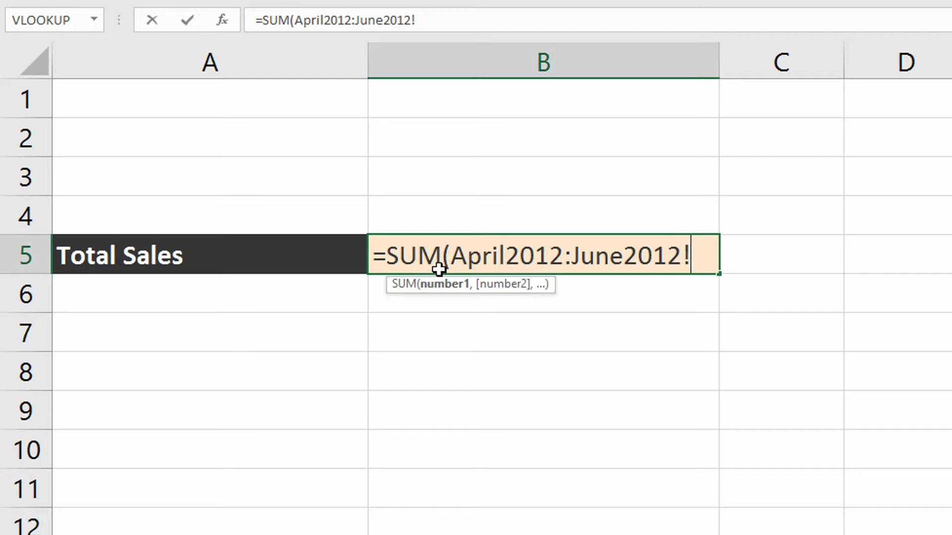
How to create a 3d reference in excel?  Excel offers a flexible approach, allowing you to include as many worksheets as your analysis demands within a single 3D reference. This flexibility ensures that you can work with extensive datasets without encountering complications. Simply separate the sheet names using a colon (:) and Excel will handle the rest, seamlessly integrating the data from multiple sheets.

Benefits of 3D References

How to create a 3d reference in excel? Now that you have a grasp of what 3D references entail, let’s delve into the multitude of advantages they offer:

1. Efficiency: By referencing data across multiple sheets, you save valuable time that would otherwise be spent on manual data consolidation.
2. Accuracy: The automation of data consolidation eliminates the possibility of manual errors, ensuring precise results.
3. Simplicity: Your formulas are streamlined, and your spreadsheets remain clutter-free, enhancing overall clarity.
4. Scalability: Whether you’re dealing with small or large datasets, 3D references handle the scale with ease.
5. Organization: You can maintain data in separate sheets based on logical categories while retaining the capability to analyze it collectively.

Common Mistakes to Avoid

Although 3D references are a potent tool, they can be somewhat challenging to use correctly. Here are some common mistakes to be vigilant about:

1. Misspelling Worksheet Names: Always double-check your worksheet names to avoid typos or errors.
2. Forgetting Quotation Marks: It’s imperative to consistently enclose the workbook name in single quotation marks.
3. Not Using Exclamation Marks: Do not overlook the importance of using an exclamation mark (!) to separate the workbook name from the reference.

Practical Example: Sales Data Analysis

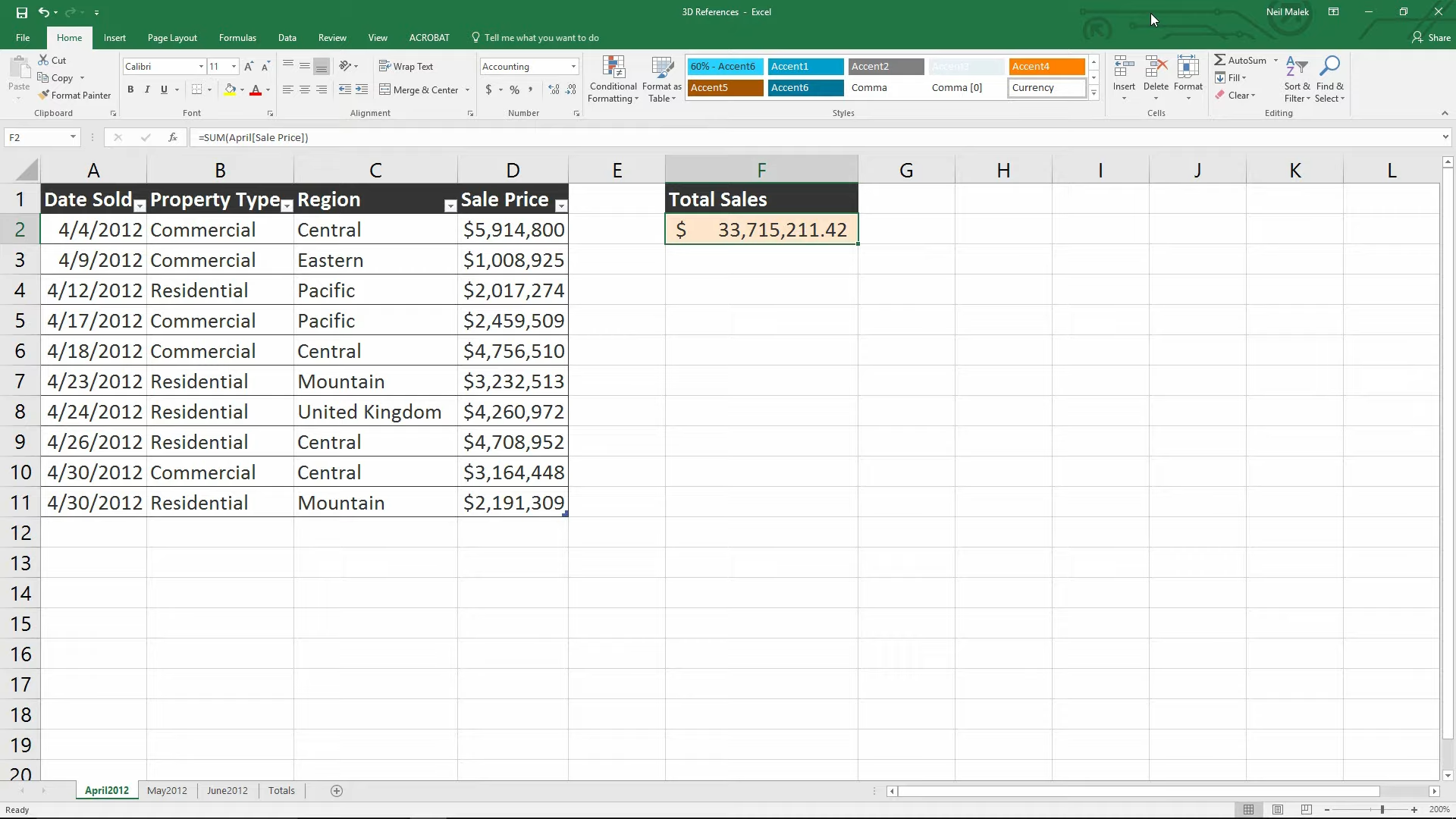
Let’s put theory into practice with a real-world scenario. Visualize that you have a workbook comprising twelve worksheets, each representing a month. Your goal is to calculate the total sales for the year. With a 3D reference, you can craft a formula like this:

=SUM('January:December'!B2)

Excel will automatically sum up cell B2 from each of these sheets, providing you with the annual total.

Tips for Efficiently Using 3D References

How to create a 3d reference in excel?  Here are some quick tips to assist you in harnessing 3D references with utmost efficiency:

1. Stay Organized: Label your worksheets effectively to ensure easy reference and navigation.
2. Use Named Ranges: Consider naming your ranges for added clarity and readability.
3. Document Your Work: Enhance the clarity of your spreadsheets by adding comments to your formulas, explaining their purpose and functionality.

Conclusion: Simplifying Data Analysis with 3D References

In conclusion, 3D references in Excel represent a potent tool for streamlining data analysis and calculations across multiple worksheets. By grasping the syntax, understanding the benefits, and being mindful of potential pitfalls, you can elevate your proficiency as an Excel user. So, the next time you find yourself grappling with complex spreadsheets, remember to leverage the magic of 3D references to simplify your tasks and enhance your productivity.

FAQs (Frequently Asked Questions)

Q1: What are 3D references used for in Excel? 3D references in Excel are employed to reference the same cell or range across multiple worksheets within a workbook. They excel at summarizing data, optimizing formulas, and simplifying intricate calculations.

Q2: How do I create a 3D reference in Excel? To craft a 3D reference in Excel, initiate it with an equal sign (=), followed by the desired function or formula, and then specify the reference to the worksheets involved. Wrap the workbook name in single quotation marks and use an exclamation mark (!) to demarcate the workbook name from the cell or range reference.

Q3: Can I use 3D references with more than two worksheets? Absolutely, you can use 3D references with as many worksheets as your analysis necessitates. Just ensure to separate the sheet names with a colon (:) within the reference.

Q4: What are some common mistakes to avoid when using 3D references? Common pitfalls to steer clear of encompass misspelling worksheet names, ensuring you enclose the workbook name in quotation marks, and always including the exclamation mark between the workbook name and the reference.

How to create a 3d reference in excel?  Now that you’ve unlocked the secrets of 3D references in Excel, you’re well on your way to becoming a proficient Excel wizard! Happy spreadsheeting!

Tags: Artificial Intelligence digital marketing Excel Primavera P6 SeminarsWorld