How to Insert Check Marks in Excel? In this blog post, we are going to show you how you can insert check marks in Excel. This is a very easy process that only takes a few steps. So, if you need to add check marks to your Excel spreadsheet, then follow these steps. If you’re already familiar with how to add check marks to Excel, then feel free to skip ahead to the instructions below. Otherwise, keep reading for more information on how to do this!

Although they might seem small and insignificant, check marks can play an important role in Excel spreadsheets. They can be used to indicate whether or not certain tasks have been completed or whether specific items are satisfactory. In some cases, they may even be required as part of a formal document or report. Whatever your reason for wanting them in your spreadsheet, adding check marks is actually a very easy process. Just follow the steps outlined below, and you’ll have them inserted in no time!

How to Insert Check Marks in Excel (In Easy Steps)

Do you need to insert check marks in Excel for a project or presentation? It’s easy to do, and this helpful guide will show you how. We’ll walk you through the steps, whether you’re using a standard Windows PC or a Mac. We’ve also included some helpful tips on formatting your check marks for the best results. Let’s get started!

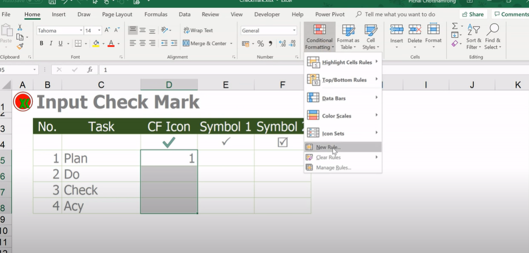
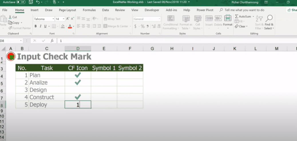
1. Open your Excel spreadsheet.

2. Click on the cell where you want to insert the check mark.

3. Go to the “Insert” tab on the ribbon.

4. In the “Symbols” group, click on the “Symbol” button.

5. This will open the “Symbol” dialog box. In the “Font” drop-down, select “Wingdings 2”.

6. Scroll down until you find the check mark character (it looks like a square with a checkmark in it). Double-click on this character to insert it into your cell.

7. Click the “Close” button to close the dialog box.

Conclusion

And that’s all there is to it! Just follow these simple steps, and you’ll be able to insert check marks into your Excel spreadsheet with ease.

You can also format your checkmark cells for different colors or font styles if you want. To do this, select the cells containing the check marks and use the options in the “Font” group on the ribbon. For example, you can change the color of the text or make it bold or italic. Experiment with different settings until you find something that looks good.

We hope this guide has helped show you how to insert check marks into Excel. If you have any questions or comments, please leave them below. And if you know of any other tips or tricks for working with check marks in Excel, be sure to share them with us!

That’s all there is to it! Just follow these simple steps, and you’ll be able to insert check marks into your Excel spreadsheet with ease. You can also format your checkmark cells for different colors or font styles if you want. To do this, select the cells containing the check marks and use the options in the “Font” group on the ribbon. For example, you can change the color of the text or make it bold or italic. Experiment with different settings until you find something that looks good.

Finally, we looked at how to change the style of your line chart in Excel. This is a great way to make your charts look more professional and visually appealing. We hope you found this tutorial helpful. Please let us know in the comments section below if you have any questions or comments.