‘How to Create a Formula in Excel’ Simplified: 5 Key Steps for Beginners
How to create a number sequence in excel formula? Excel’s capability to perform calculations using formulas is what sets it apart as a powerful tool for data analysis and management. For beginners, mastering how to create a formula in Excel can seem overwhelming at first. However, breaking down the process into manageable steps can simplify learning. This article expands on the five key steps to create formulas in Excel, complete with detailed explanations and examples to guide you through each stage.
Table of Contents
1. Understanding the Basics of Excel Formulas
How to Create a Formula in Excel? The foundation of using Excel efficiently lies in understanding how formulas work. Formulas are expressions that calculate values, using a combination of numbers, cell references, and operators. The fundamental concepts include:
- Equal Sign (
=): Every formula begins with an=, signaling Excel to perform a calculation. - Operators: These symbols dictate the operation type. Basic arithmetic operators include addition (
+), subtraction (-), multiplication (*), and division (/). - Cell References: Instead of typing numbers directly into a formula, use cell references (like
A1) to point to the specific data. This approach makes your formulas dynamic and adaptable to data changes.
Example: To add two numbers located in cells A1 and A2, you would enter =A1+A2 in the cell where you want the result to appear.
2. Entering Your First Formula
Creating a formula in Excel is straightforward:
- Select a Cell: Choose the cell where you want the formula’s result displayed.
- Initiate the Formula: Type an
=to start. - Construct Your Formula: Input the calculation by combining cell references and operators. For instance,
=A1-B1subtracts the value in B1 from A1. - Execute: Press Enter, and Excel computes the formula, showing the outcome in the selected cell.
Example: If A1 has 10 and B1 has 5, entering =A1-B1 and pressing Enter will display the result 5 in the chosen cell.
3. Using Cell References Effectively
Cell references are pivotal in making your Excel workbooks dynamic. There are two types:
- Relative References adjust based on the formula’s location. If you copy
=A1+B1from C1 to C2, it automatically changes to=A2+B2. - Absolute References remain unchanged when copied or moved. Denoted by
$(e.g.,$A$1), if you copy=$A$1+$B$1from C1 to C2, the formula stays the same, always referencing A1 and B1.
Example: For a consistent addition of A1 to various cells, use an absolute reference like =$A$1+B1. Copying this down a column will add A1’s value to each cell in column B.
4. Incorporating Functions into Formulas
Functions are built-in formulas that simplify complex calculations. They follow a specific syntax: a function name followed by arguments in parentheses.
- Syntax:
=FUNCTION_NAME(argument1, argument2, ...) - Common Functions:
- SUM: Adds a range of cells,
=SUM(A1:A5)adds the values from A1 to A5. - AVERAGE: Calculates the average of a range,
=AVERAGE(B1:B5)gives the average of values in cells B1 through B5.
- SUM: Adds a range of cells,
Example: To calculate the total of sales in cells A1 through A10, use =SUM(A1:A10). Excel adds up all the numbers in the specified range and displays the total.
5. Debugging and Error-Checking Your Formulas
Errors can occur, but Excel provides tools to help identify and fix them:
- Error Messages: Symbols like
#DIV/0!indicate issues. Hover over the cell for tips on resolution. - Formula Auditing Tools: Under the Formulas tab, these tools can trace precedents, show calculations step by step, and highlight errors, aiding in troubleshooting.
Example: If =A1/B1 results in #DIV/0!, it means B1 is zero or empty. Checking the cell’s value or using auditing tools can help identify and rectify such issues.
How do I create an automatic formula in Excel?
Excel provides an incredible feature called “AutoSum” that makes creating automatic formulas a breeze:
1. Select the Target Cell
Choose the cell where you want the result of your automatic formula to appear. This could be a cell immediately below a column of numbers you want to sum, for example.
2. Click on AutoSum
In the Excel ribbon, locate the “AutoSum” button (Σ) and click on it. Excel will automatically select a range of cells above your target cell, assuming it’s appropriate for your calculation.
3. Adjust the Range
If Excel’s selection doesn’t match your intended range, simply click and drag to adjust it. You can also manually enter the range in the formula bar.
4. Press Enter
Once you’re satisfied with the selected range, press Enter. Excel will calculate the sum and display it in the target cell.
AutoSum is a quick and convenient way to create automatic formulas in Excel, saving you time and effort.
How do I create a formula in Excel table?
Excel tables are a great way to organize and analyze data. To create a formula within an Excel table, follow these steps:
1. Create a Table
Select the range of cells that you want to convert into a table. Then, go to the “Insert” tab in the Excel ribbon and click on “Table.” Excel will prompt you to confirm the range; ensure the “My table has headers” option is checked if your data has headers.
2. Enter Your Formula
Now that you have a table, you can easily create a formula. Select the cell where you want the result, type your formula, and press Enter. Excel will automatically apply the formula to the entire column in the table, adjusting for each row.
3. Utilize Table References
When creating your formula, you can reference table columns using structured references, making your formulas more dynamic and readable. For example, to sum values in a column named “Sales,” you can use the formula: =SUM(Table1[Sales]).
Excel tables offer a structured and organized way to work with formulas, ensuring consistency and accuracy in your calculations.
How to create a number sequence in excel formula?
How to create a number sequence in excel formula? Creating a number sequence in Excel using a formula can be done in several ways, depending on your specific requirements. Here are three common methods:
Method 1: Using the ROW Function
The ROW function returns the row number of a cell. By using this function, you can create a simple number sequence in Excel. Here’s how:
- In an empty column, select the cell where you want the sequence to start.
- Enter the formula
=ROW(). This formula will return the current row number. - Press Enter.
- Click and drag the fill handle (a small square at the bottom-right corner of the selected cell) down to fill the desired number of cells with the sequence.
This method will create a sequence of numbers starting from the row where you entered the formula and incrementing by one for each row.
Method 2: Using the SEQUENCE Function (Excel 365)
If you’re using Excel 365 or later versions, you can use the SEQUENCE function, which is designed for generating sequences of numbers. Here’s how:
- Select the cell where you want the sequence to start.
- Enter the formula
=SEQUENCE(number_of_rows, number_of_columns, start_value, step). Replacenumber_of_rowswith the total number of rows you want in your sequence,number_of_columnswith the number of columns (usually 1 for a simple sequence),start_valuewith the first number in the sequence, andstepwith the interval between numbers. - Press Enter.
This method allows you to create more complex sequences with custom starting values and step increments.
Method 3: Using Concatenation and ROW Function
If you want to create a sequence with a specific pattern, you can use concatenation along with the ROW function. Here’s an example of a patterned sequence:
- In an empty column, select the cell where you want the sequence to start.
- Enter the formula
="Prefix" & (ROW() - start_row + 1) & "Suffix". Replace"Prefix"and"Suffix"with your desired text, andstart_rowwith the row where you want the sequence to start. - Press Enter.
- Click and drag the fill handle down to fill the desired number of cells with the sequence.
This method allows you to create a sequence that combines text and numbers.
Choose the method that best suits your needs, and you can easily create number sequences in Excel using formulas.
Streamline Software Development with Generative AI – projectcubicle
How can I create my own formula?
Creating your own formulas in Excel is a valuable skill. Here’s a step-by-step guide to get you started:
1. Identify Your Calculation
Begin by identifying the calculation you need. Whether it’s basic arithmetic, statistical analysis, or complex financial modeling, Excel can handle a wide range of calculations.
2. Learn Excel Functions
Familiarize yourself with Excel’s built-in functions. These functions can simplify your formulas and provide accurate results. Some commonly used functions include SUM, AVERAGE, MAX, and MIN.
3. Write Your Formula
In an empty cell, start writing your formula. Use appropriate functions, cell references, and operators to express your calculation. Excel’s formula bar is where you’ll enter your formula.
4. Test and Refine
After entering your formula, test it with sample data to ensure it produces the desired results. If needed, refine your formula by adjusting references or functions.
5. Apply the Formula
Once your formula is ready, you can apply it to multiple cells or use it as a template for similar calculations throughout your spreadsheet.
Creating your own formulas in Excel empowers you to tailor your calculations to specific requirements, making your data analysis more efficient.
How do I create a formula for an entire column in Excel?
Creating a formula that applies to an entire column in Excel can save you time and effort when working with large datasets. Here’s how you can do it:
1. Select the Cell
Choose the cell in the column where you want the formula to start. This cell will be the reference point for your formula.
2. Write the Formula
In the selected cell, write your formula as you normally would, making sure to use relative cell references. For example, if you want to calculate the percentage in each row of a column, your formula could be: =A2/B2.
3. Apply the Formula
After writing the formula, press Enter. Excel will calculate the result for that specific cell.
4. Autofill the Formula
To apply the formula to the entire column, hover over the small square in the bottom-right corner of the selected cell (the fill handle). When the cursor changes to a black cross, click and drag it down the column. Excel will autofill the formula for all the cells in the column, adjusting the references accordingly.
Creating a formula for an entire column is a powerful way to automate calculations across large datasets.
Atomic Habits That Will Make You Stand Out in Business Life: 5 Steps, 5 Gains – projectcubicle
How to Create a Formula in Excel Conclusion
Mastering how to create a formula in Excel is essential for anyone looking to leverage Excel’s full capabilities. By starting with basic operations, understanding cell references, incorporating functions, and learning to debug, beginners can build a solid foundation in Excel. Practice is key; experiment with different formulas, functions, and datasets to become proficient. Remember, the more you practice, the more intuitive and powerful your Excel skills will become, opening up endless possibilities for data analysis and management.
How to Create a Formula in Excel FAQs
Q: Can I use Excel functions in my custom formulas? Yes, Excel functions can be incorporated into your custom formulas, allowing you to perform complex calculations.
Q: What if I make a mistake in my formula? If you make an error in your formula, Excel will display an error message. Double-check your formula for typos, incorrect references, or missing operators.
Q: Are there shortcuts for creating formulas in Excel? Certainly! Excel offers various keyboard shortcuts and quick methods to create formulas. For example, you can press “Alt + =” to automatically sum a range of numbers.
Q: Can I nest functions within my formulas? Yes, you can nest functions by using one function’s result as an argument in another function. This allows you to create intricate calculations.
Q: How do I troubleshoot formula errors? If you encounter formula errors, Excel provides error-checking tools to help you identify and fix the issue. Review the formula for common mistakes, and use the error messages as clues to pinpoint the problem.
Q: Can I use cell references from different sheets in my formulas? Yes, you can reference cells from other sheets by specifying the sheet name followed by an exclamation mark (!) before the cell reference (e.g., ‘Sheet2’!A1).

Daily motivation for projectcubicle.com
Hello, I’m Cansu, a professional dedicated to creating Excel tutorials, specifically catering to the needs of B2B professionals. With a passion for data analysis and a deep understanding of Microsoft Excel, I have built a reputation for providing comprehensive and user-friendly tutorials that empower businesses to harness the full potential of this powerful software.
I have always been fascinated by the intricate world of numbers and the ability of Excel to transform raw data into meaningful insights. Throughout my career, I have honed my data manipulation, visualization, and automation skills, enabling me to streamline complex processes and drive efficiency in various industries.
As a B2B specialist, I recognize the unique challenges that professionals face when managing and analyzing large volumes of data. With this understanding, I create tutorials tailored to businesses’ specific needs, offering practical solutions to enhance productivity, improve decision-making, and optimize workflows.
My tutorials cover various topics, including advanced formulas and functions, data modeling, pivot tables, macros, and data visualization techniques. I strive to explain complex concepts in a clear and accessible manner, ensuring that even those with limited Excel experience can grasp the concepts and apply them effectively in their work.
In addition to my tutorial work, I actively engage with the Excel community through workshops, webinars, and online forums. I believe in the power of knowledge sharing and collaborative learning, and I am committed to helping professionals unlock their full potential by mastering Excel.
With a strong track record of success and a growing community of satisfied learners, I continue to expand my repertoire of Excel tutorials, keeping up with the latest advancements and features in the software. I aim to empower businesses with the skills and tools they need to thrive in today’s data-driven world.
Suppose you are a B2B professional looking to enhance your Excel skills or a business seeking to improve data management practices. In that case, I invite you to join me on this journey of exploration and mastery. Let’s unlock the true potential of Excel together!
https://www.linkedin.com/in/cansuaydinim/


