Weibull Distribution in Excel: Can Excel do Weibull analysis?

In the realm of statistical analysis, the WEIBULL.DIST stands out for its versatility in modeling life data, particularly in reliability engineering and failure time analysis. For instance, a common Weibull distribution example might involve analyzing the lifespan of mechanical components to predict failure rates, which is invaluable for maintenance planning and quality control. Conducting such analysis is not limited to Excel; Weibull distribution in MATLAB offers advanced functionalities for more sophisticated data analysis, including fitting and visualization tools that can handle complex datasets with ease. However, for many users, conducting a Weibull in Excel example offers a more accessible entry point into reliability analysis. Excel users can perform these analyses by learning how to calculate alpha and beta for Weibull distribution in Excel, which are the distribution’s shape and scale parameters, respectively. Fortunately, numerous resources, including Weibull Excel spreadsheet download options, are available online, providing templates and examples that simplify these calculations. Working through Weibull distribution example problems allows analysts to gain practical experience with the distribution, enhancing their ability to model and interpret reliability data effectively.

Can Excel do Weibull analysis? The Weibull Distribution stands as a pivotal statistical tool, especially within the realms of reliability engineering and life data analysis. Its utility in predicting the time until a specific event, such as the failure of a mechanical component, renders it indispensable for professionals striving to enhance product durability and performance. Excel, with its comprehensive suite of analytical tools, facilitates the application of Weibull Distribution, empowering users to perform intricate data analysis and reliability assessments with relative ease.

Step-by-Step Guide to Utilizing Weibull.Dist Function

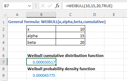
Delving into Excel to perform Weibull Distribution analysis begins with understanding the WEIBULL.DIST function. This function (WEIBULL.DIST) demands four arguments: the value at which to evaluate the function (x), the shape parameter (alpha), the scale parameter (beta), and a logical flag indicating whether to calculate the PDF or CDF. The syntax appears as =WEIBULL.DIST(x, alpha, beta, TRUE/FALSE), where setting the last parameter to TRUE calculates the CDF, and FALSE calculates the PDF.

Table of Contents

For instance, if tasked with analyzing the reliability of a new gadget, one would collect data on its operational lifespan until failure. This data becomes the foundation for the Weibull analysis in Excel. By inputting the lifespan data as ‘x’ and estimating suitable values for alpha and beta, analysts can predict the failure rate over time. This predictive capability is instrumental in preemptive maintenance scheduling and enhancing product design for future iterations.

Weibull analysis in Excel

Visualizing Weibull Distribution

Beyond numerical analysis, visual representation of Weibull Distribution (WEIBULL.DIST) in Excel can significantly augment comprehension and presentation of results. After calculating the necessary Weibull parameters and their corresponding values, plotting these against the lifespan data on a chart elucidates trends and patterns that might be obscure in raw data form. Excel charts offer a dynamic way to showcase the distribution curve, highlighting areas of interest such as the mean time to failure or the point at which the failure rate accelerates.

Creating a chart involves selecting the calculated Weibull values alongside the original data points. The resulting graph provides a visual summary of the analysis, facilitating discussions among stakeholders about product reliability and necessary improvements. This graphical approach not only simplifies complex statistical concepts but also enhances decision-making processes by providing a clear, intuitive understanding of the data.

Advanced Analysis: Parameter Estimation

A crucial aspect of Weibull Distribution in Excel is the estimation of the alpha and beta parameters, which significantly influence the accuracy of the analysis. Excel’s Solver feature can optimize these parameters to fit the collected data best. This process involves setting up an objective function, such as minimizing the sum of squared errors between the observed and model-predicted values, and using Solver to adjust alpha and beta to meet this objective.

Parameter estimation might seem daunting due to its mathematical underpinnings, but Excel’s Solver simplifies this process, making it accessible even to those with a limited statistical background. Accurate estimation of Weibull parameters ensures the reliability model closely mirrors real-world behavior, thereby providing more dependable predictions and insights.

Applying Weibull Analysis in Real-World Scenarios

The applicability of Weibull Distribution in Excel extends beyond theoretical exercises; it’s a practical tool for myriad real-world applications. From forecasting the lifespan of industrial machinery to determining the failure rates of consumer electronics, Weibull analysis offers invaluable insights that drive informed decision-making. For reliability engineers, it’s a cornerstone methodology for designing robust systems and establishing effective maintenance strategies.

Moreover, Weibull analysis (WEIBULL.DIST) is not confined to engineering disciplines. It finds relevance in financial risk assessment, healthcare prognosis models, and even in meteorological predictions, showcasing its versatility and adaptability across sectors. The ability to model and predict time-to-event data accurately is a powerful asset in any data analyst’s toolkit, facilitated by the robust functionalities of Excel (WEIBULL.DIST).

Understanding Weibull Distribution Formula with a Concrete Example

The Weibull Distribution Formula plays a pivotal role in reliability engineering. Let’s consider an example where you’re tasked with analyzing the failure rate of a new type of battery. The formula f(x; α, β) = (α/β) * (x/β)^(α-1) * exp(-(x/β)^α) becomes the foundation of your analysis. Suppose you have failure data for 100 batteries with α (shape parameter) estimated at 1.5 and β (scale parameter) at 2000 hours. Using Excel, you input these parameters into the WEIBULL.DIST function to predict the probability of failure over time, allowing for strategic planning around warranty periods or maintenance schedules.

Exponential Smoothing in Excel: Forecasting Techniques – projectcubicle

Applying WEIBULL.DIST in Excel: A Step-by-Step Guide

Imagine you’re examining the lifespan of LED lightbulbs. You have recorded the hours until failure for a sample of 50 bulbs. Here’s how you might proceed:

Collect Data: Your dataset includes hours until failure: 1000, 1500, 2000, etc.
Estimate Parameters: Initially, you estimate α at 2.5 and β at 1800.
Use Excel: In Excel, you’d input =WEIBULL.DIST(x, 2.5, 1800, FALSE) for each data point x to get the PDF or TRUE for the CDF.
Analyze Results: The output helps you visualize the failure distribution, guiding decisions on product improvement.

This Weibull in Excel Example demonstrates Excel’s utility in transforming raw data into actionable insights.

Weibull Distribution in MATLAB vs. Excel: An Illustrative Comparison

Weibull Distribution in MATLAB (Weibull distribution – matlab) offers advanced functionalities, such as fitting data to a Weibull distribution (Weibull distribution – matlab) with wblfit and generating plots with wblplot. For a comparative analysis, let’s say you’re assessing the durability of solar panels. In MATLAB (Weibull distribution – matlab), you’d use wblfit to find α and β, then wblplot to visualize the fit. Replicating this in Excel involves using WEIBULL.DIST chart features to plot the distribution. Although MATLAB (Weibull distribution – matlab) provides more detailed statistical tools, Excel’s approach is more accessible for those without a background in programming, making it a valuable alternative for conducting preliminary analyses.

How to Calculate Alpha and Beta for Weibull Distribution in Excel: Illustrated Guide

Calculating α (alpha) and β (beta) in Excel can seem daunting. Here’s a simplified example: Suppose you’re evaluating the failure times of a set of pumps. After plotting your data on a Weibull plot, you guess initial values of α at 1.8 and β at 300 hours. Using Excel’s Solver, you adjust these values to minimize the sum of squared differences between your observed and the Weibull model’s predicted failure rates. This iterative process hones in on the most accurate α and β, enhancing your model’s predictive power.

Weibull in Excel Example with Spreadsheet Download for Enhanced Learning

Providing a Weibull in Excel Example with a spreadsheet download can significantly expedite the learning curve. Imagine a spreadsheet template with predefined formulas where users only need to input their failure time data. For instance, a user analyzing the reliability of HVAC systems in commercial buildings could input their system failure data into the spreadsheet and immediately receive a Weibull analysis, including estimated α and β parameters and a graphical representation of the distribution. This hands-on approach demystifies Weibull analysis, making it approachable for practitioners across industries.

Tackling Weibull Distribution Example Problems for Practical Mastery

Let’s solve a Weibull Distribution Example Problem to consolidate our understanding. Consider a scenario where a manufacturing company wants to assess the failure rate of its conveyor belts. The data collected represents the number of days until failure for 30 belts. Using the steps outlined for Excel analysis (WEIBULL.DIST), the company can determine the Weibull parameters, α and β, providing insights into the belts’ expected lifespan and identifying any potential for improvements.

People Also Ask About Weibull Analysis:

Can Excel do Weibull analysis?

Absolutely. Excel can conduct Weibull analysis using the WEIBULL.DIST function.

How do you generate a random Weibull distribution in Excel?

To generate a random Weibull distribution in Excel, you can use the WEIBULL.DIST function in combination with the RAND() function. However, for generating random numbers directly from a Weibull distribution, Excel does not have a built-in function like RAND() that directly outputs Weibull distributed numbers. Instead, you can use the inverse transformation method with the WEIBULL.INV function. Here’s an example (weibull distribution example) formula:

=WEIBULL.INV(RAND(), alpha, beta)

This formula generates a random number based on the Weibull distribution with specified shape (alpha) and scale (beta) parameters.

where:

f(x; α, β) is the probability density function (PDF) of the distribution,
x is the time to failure,
α (alpha) is the shape parameter, which dictates the failure rate’s behavior over time,
β (beta) is the scale parameter, which stretches or compresses the distribution on the horizontal axis.

What are the three parameters of Weibull in Excel?

In Excel, the Weibull distribution primarily involves two parameters when using the WEIBULL.DIST function: alpha (shape parameter) and beta (scale parameter). The third parameter in some contexts, referred to when discussing the generalized or three-parameter Weibull distribution, includes a location parameter γ (gamma), which shifts the distribution left or right on the horizontal axis. However, Excel’s WEIBULL.DIST function does not directly incorporate this third parameter; analysis involving it requires additional calculations.

Motivation

Cansu Aydin

Hello, I’m Cansu, a professional dedicated to creating Excel tutorials, specifically catering to the needs of B2B professionals. With a passion for data analysis and a deep understanding of Microsoft Excel, I have built a reputation for providing comprehensive and user-friendly tutorials that empower businesses to harness the full potential of this powerful software.

I have always been fascinated by the intricate world of numbers and the ability of Excel to transform raw data into meaningful insights. Throughout my career, I have honed my data manipulation, visualization, and automation skills, enabling me to streamline complex processes and drive efficiency in various industries.

As a B2B specialist, I recognize the unique challenges that professionals face when managing and analyzing large volumes of data. With this understanding, I create tutorials tailored to businesses’ specific needs, offering practical solutions to enhance productivity, improve decision-making, and optimize workflows.

My tutorials cover various topics, including advanced formulas and functions, data modeling, pivot tables, macros, and data visualization techniques. I strive to explain complex concepts in a clear and accessible manner, ensuring that even those with limited Excel experience can grasp the concepts and apply them effectively in their work.

In addition to my tutorial work, I actively engage with the Excel community through workshops, webinars, and online forums. I believe in the power of knowledge sharing and collaborative learning, and I am committed to helping professionals unlock their full potential by mastering Excel.

With a strong track record of success and a growing community of satisfied learners, I continue to expand my repertoire of Excel tutorials, keeping up with the latest advancements and features in the software. I aim to empower businesses with the skills and tools they need to thrive in today’s data-driven world.

Suppose you are a B2B professional looking to enhance your Excel skills or a business seeking to improve data management practices. In that case, I invite you to join me on this journey of exploration and mastery. Let’s unlock the true potential of Excel together!

https://www.linkedin.com/in/cansuaydinim/