Excel Hide Shortcut: Boosting Your Productivity with Hidden Features
Discover the Excel hide shortcut and unleash the hidden potential of Microsoft Excel. Enhance your productivity and efficiency with this powerful tool. Learn about the shortcuts, tips, and tricks to navigate and hide data effortlessly.
Table of Contents
Introduction: Unlocking the Power of Excel Hide Shortcut
When it comes to managing and organizing data, Microsoft Excel is a trusted companion for professionals across various industries. However, many users remain unaware of the plethora of features and shortcuts available that can significantly boost productivity. This article will dive into the Excel hide shortcut, a powerful tool that allows you to effortlessly hide data, columns, and rows. By mastering this shortcut, you can streamline your workflow, declutter your spreadsheets, and focus on the information that matters most.
Excel Hide Shortcut: The Key to Efficiency
Excel offers a range of shortcuts to help users navigate through complex spreadsheets with ease. One such shortcut is the Excel hide shortcut, which enables you to hide selected data, columns, or rows in just a few keystrokes. By utilizing this shortcut effectively, you can declutter your spreadsheet, focus on relevant information, and improve overall efficiency. Let’s explore how to use the Excel hide shortcut to its full potential.
How to Use the Excel Hide Shortcut?
Step 1: Select the Data to Hide
To begin, select the data you want to hide. You can do this by clicking and dragging your cursor over the desired cells, columns, or rows. Alternatively, you can press Ctrl and click on individual cells, columns, or rows to select multiple non-adjacent elements.
Step 2: Apply the Hide Shortcut
Once you have made your selection, press the Ctrl and 0 (zero) keys simultaneously. Voila! The selected data will disappear from view, making your spreadsheet cleaner and more focused. Don’t worry; the hidden data is not deleted and can be easily restored.
Frequently Asked Questions about Excel Hide Shortcut
1. Can I hide multiple columns or rows simultaneously using the Excel hide shortcut?
Yes, absolutely! The Excel hide shortcut allows you to select and hide multiple columns or rows simultaneously. Simply select the desired columns or rows and apply the hide shortcut (Ctrl + 0).
2. How can I unhide hidden data in Excel?
Unhiding hidden data in Excel is just as simple as hiding it. To unhide hidden columns, select the adjacent columns, right-click, and choose “Unhide.” For unhiding hidden rows, select the adjacent rows, right-click, and select “Unhide.” You can also use the shortcut Alt + Shift + 0 (zero) to unhide both columns and rows simultaneously.
3. Can I use Excel to hide a shortcut in protected sheets?
Unfortunately, the Excel hide shortcut cannot be used on protected sheets. To hide data in a protected sheet, you will need to unprotect the sheet first, apply the hidden shortcut, and then protect the sheet again.
4. Is there a way to hide formulas in Excel?
You can hide formulas in Excel by utilizing the “Format Cells” option. Select the cells containing the formulas, right-click, choose “Format Cells,” go to the “Protection” tab, and check the “Hidden” box. After clicking “OK,” the formulas will be hidden from view, but the results will still be visible.
5. How can I quickly unhide all hidden columns and rows in Excel?
To unhide all hidden columns and rows in Excel, you can use the following shortcut: Ctrl + Shift + 8. This command will reveal all hidden elements in your spreadsheet instantly.
Tips and Tricks to Maximize Productivity with Excel Hide Shortcut
Now that you are familiar with the Excel hide shortcut let’s explore some additional tips and tricks to maximize your productivity:
1. Grouping and Outlining
Excel allows you to group and outline data, providing a structured view of your spreadsheet. By grouping related columns or rows, you can quickly hide or unhide entire sections with a single click. To group columns or rows, select them, right-click, and choose “Group.” You can then use the “+” or “-” signs to expand or collapse the grouped sections.
2. Customizing Hidden Data Appearance
When you hide data in Excel, the hidden cells are displayed with a small triangle in the top-left corner. However, you can customize the appearance of hidden data to make it more visually distinct. Go to the “File” tab, select “Options,” choose the “Advanced” tab, and under the “Display options for this workbook” section, check the “Show outline symbols if an outline is applied” box.
3. Using Keyboard Shortcuts for Efficient Navigation
In addition to the Excel hide shortcut, several other keyboard shortcuts can enhance your navigation within a spreadsheet. For example, pressing Ctrl + Arrow keys allows you to quickly move to the edge of a range, while Ctrl + Home takes you to the top-left cell of the sheet. Combined with the Excel hide shortcut, these shortcuts enable seamless navigation and data manipulation.
4. Hiding and Unhiding Sheets
Apart from hiding data within a sheet, Excel also allows you to hide and unhide entire sheets. Right-click on the sheet name, choose “Hide” to hide the sheet, and “Unhide” to reveal it again. This feature is useful when working with large workbooks or when you want to focus on specific sheets temporarily.
5. Protecting Hidden Data
You can protect your Excel workbook to prevent accidental changes to hidden data. By setting a password, you can ensure that only authorized individuals can unhide and modify hidden data. To protect your workbook, go to the “Review” tab, click on “Protect Workbook,” and follow the instructions.
6. Automating Hide and Unhide Actions with Macros
You can save time by creating macros if you frequently hide and unhide specific sections in your Excel worksheets. Macros allow you to automate repetitive tasks, including hiding and unhiding data. By recording a macro that applies the hide or unhides action, you can assign it to a keyboard shortcut or a button, making the process even more efficient.
Conclusion: Embrace the Power of Excel Hide Shortcut
The Excel hide shortcut is a valuable tool that empowers users to efficiently manage and declutter their spreadsheets. By leveraging this feature, you can easily hide and unhide data, columns, rows, and even entire sheets, streamlining your workflow and improving productivity. Remember to explore the additional tips and tricks mentioned in this article to maximize the potential of the Excel hide shortcut. With practice and familiarity, you’ll become a master of Excel’s hidden features, unlocking a new level of efficiency in your Excel workflow. From grouping and outlining to customizing the appearance of hidden data, there are various techniques you can employ to enhance your experience with Excel.
In this article, we have delved into the Excel hide shortcut, guiding you through its usage and providing valuable tips and tricks. By incorporating these techniques into your daily Excel usage, you can save time, reduce clutter, and focus on the most relevant data for your tasks.
In conclusion, mastering the Excel hide shortcut is a game-changer for anyone working with data in Excel. Whether you’re organizing large datasets, creating reports, or simply managing your personal finances, this powerful tool will enable you to hide and unhide data effortlessly. Remember to utilize additional features like grouping, customizing hidden data appearance, and leveraging keyboard shortcuts for efficient navigation.
So, why wait? Start exploring the Excel hide shortcut today and witness the transformation it brings to your productivity and workflow. Embrace the hidden potential of Excel and discover a world of possibilities that lie beneath the surface.
Hello, I’m Cansu, a professional dedicated to creating Excel tutorials, specifically catering to the needs of B2B professionals. With a passion for data analysis and a deep understanding of Microsoft Excel, I have built a reputation for providing comprehensive and user-friendly tutorials that empower businesses to harness the full potential of this powerful software.
I have always been fascinated by the intricate world of numbers and the ability of Excel to transform raw data into meaningful insights. Throughout my career, I have honed my data manipulation, visualization, and automation skills, enabling me to streamline complex processes and drive efficiency in various industries.
As a B2B specialist, I recognize the unique challenges that professionals face when managing and analyzing large volumes of data. With this understanding, I create tutorials tailored to businesses’ specific needs, offering practical solutions to enhance productivity, improve decision-making, and optimize workflows.
My tutorials cover various topics, including advanced formulas and functions, data modeling, pivot tables, macros, and data visualization techniques. I strive to explain complex concepts in a clear and accessible manner, ensuring that even those with limited Excel experience can grasp the concepts and apply them effectively in their work.
In addition to my tutorial work, I actively engage with the Excel community through workshops, webinars, and online forums. I believe in the power of knowledge sharing and collaborative learning, and I am committed to helping professionals unlock their full potential by mastering Excel.
With a strong track record of success and a growing community of satisfied learners, I continue to expand my repertoire of Excel tutorials, keeping up with the latest advancements and features in the software. I aim to empower businesses with the skills and tools they need to thrive in today’s data-driven world.
Suppose you are a B2B professional looking to enhance your Excel skills or a business seeking to improve data management practices. In that case, I invite you to join me on this journey of exploration and mastery. Let’s unlock the true potential of Excel together!
https://www.linkedin.com/in/cansuaydinim/


