Excel Bar Chart: A Complete Guide for Beginners

Are you looking for a simple yet effective way to represent your data visually? Excel Bar Chart is the perfect solution for you. In this article, we will guide you through the process of creating a bar chart in Excel and provide you with tips to make it look professional. So, let’s get started!

Introduction

Excel Bar Chart is a powerful tool that helps you to visualize data in a way that is easy to understand. With just a few clicks, you can create a chart that displays your data in columns or bars, making it easier to compare values. A bar chart is a great way to show changes in data over time, compare two or more data sets, or illustrate relationships between different data points.

Benefits of Using Excel Bar Chart

1. Helps to visualize data in a clear and concise manner.
2. Provides an easy way to compare data points.
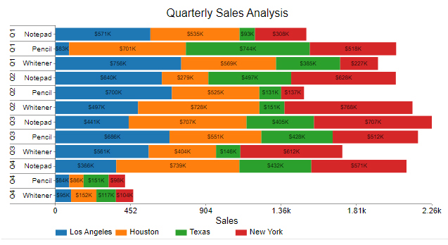
3. Can display multiple data sets in a single chart.
4. Allows for customization of chart appearance to match your preferences.

Creating an Excel Bar Chart

To create an Excel Bar Chart, follow these simple steps:

1. Open Excel and enter your data in a table format.
2. Select the cells containing the data you want to chart.
3. Click on the ‘Insert’ tab in the ribbon.
4. Click on the ‘Bar Chart’ icon.
5. Select the type of chart you want to create.
6. Customize the chart appearance by adding titles, labels, and formatting options.

Tips for Creating a Professional-Looking Excel Bar Chart

1. Use appropriate chart types based on your data.
2. Keep your chart simple and easy to read.
3. Label your chart axes and data points clearly.
4. Choose a color scheme that is easy on the eyes.
5. Use consistent formatting throughout your chart.

Additional Tips for Creating Effective Excel Bar Charts

Here are some additional tips to help you create effective Excel Bar Charts:

1. Use the appropriate chart type: Depending on your data, you may want to use a clustered, stacked, or 100% stacked bar chart. Choose the type that best suits your data and allows for easy comparison.
2. Use contrasting colors: Use colors that contrast well with each other to make your data stand out. Avoid using too many colors, which can make the chart look cluttered.
3. Use descriptive labels: Label your axes and data points in a way that accurately reflects your data. Use descriptive labels that are easy to understand.
4. Use data markers: Use data markers to highlight specific data points or trends in your chart. This can make your data easier to interpret.
5. Use a chart title: Add a descriptive chart title that summarizes the data being presented. This can help viewers quickly understand the purpose of the chart.
6. Use gridlines: Use gridlines to make it easier to read and compare the data in your chart. Be sure to adjust the gridline spacing to suit your data.

Common Mistakes to Avoid While Creating Excel Bar Charts

Creating an Excel Bar Chart is easy, but you should avoid some common mistakes to ensure that your chart looks professional and communicates your data accurately.

1. Choosing the wrong chart type: Be sure to select the appropriate one based on your data. For example, if you want to compare two or more data sets, a clustered bar chart is a better choice than a stacked bar chart.
2. Cluttered chart: Avoid cluttering your chart with too much data or formatting options. Keep it simple and easy to read.
3. Unclear labeling: Make sure your chart axes and data points are clearly labeled. Unclear labeling can cause confusion and misinterpretation of your data.
4. Poor color choice: Choose a color scheme that is easy on the eyes and contrasts well with your data. Avoid using too many colors or a distracting color scheme.
5. Inconsistent formatting: Use consistent formatting throughout your chart, including font size, colors, and label placement.

Conclusion

Excel Bar Chart is a great tool for visualizing data clearly and concisely. With the tips provided in this article, you can create a professional-looking chart that effectively communicates your data. Remember to avoid common mistakes, keep your chart simple, and customize it to your preferences. So, go ahead and create your Excel Bar Chart today!

Excel Bar Chart FAQS

Q1. Can I change the chart type after creating a Chart?

Yes, you can easily change the chart type after creating an Excel Bar Chart. To do so, select the chart and click on the ‘Design’ tab in the ribbon. Click on the ‘Change Chart Type’ icon and select the chart type you want to change to.

Q2. How do I add data labels to my Chart?

Select the chart to add data labels to your Excel Bar Chart and click on the ‘Layout’ tab in the ribbon. Click on the ‘Data Labels’ icon and select the location of the labels.

Q3. Can I customize the appearance of my Chart?

Yes, you can customize the appearance of your Excel Bar Chart. To do so, select the chart and click on the ‘Format’ tab in the ribbon. You can change the chart style, color scheme and add titles and labels.

Q4. How do I add a trendline to my Chart?

To add a trendline to your Chart, select the chart and click on the ‘Layout’ tab in the ribbon. Click on the ‘Trendline’ icon and select the type of trendline you want to add.

Q5. How can I sort my Excel Bar Chart data in ascending or descending order?

Select the chart to sort your Chart data in ascending or descending order and click on the ‘Data’ tab in the ribbon. Click on the ‘Sort’ icon and select the order you want to sort your data.