Conditional formatting is a powerful feature in Microsoft Excel that allows you to format cells based on specific criteria. This feature can be useful for identifying data trends, highlighting important information, and making your spreadsheets easier to read.

Understanding Conditional Formatting Formulas

Conditional formatting in Excel works by using formulas that evaluate each cell’s value and determine whether it meets a specified condition. These formulas can be simple, such as checking whether a cell is greater than a certain value, or complex, such as using nested IF statements to evaluate multiple conditions.

How to Apply Conditional Formatting with Formulas in Excel

Applying conditional formatting with formulas in Excel is relatively easy. Here are a few common examples:

1. a. Highlight cells greater than a certain value: To highlight cells that are greater than a certain value, select the cells you want to format, click on the “Conditional Formatting” button in the “Home” tab, and select “Highlight Cell Rules” > “Greater Than.” Enter the value you want to use as the threshold and choose a formatting style.
2. b. Highlight cells containing specific text: To highlight cells that contain specific text, select the cells you want to format, click on the “Conditional Formatting” button, and select “Highlight Cell Rules” > “Text that Contains.” Enter the text you want to search for and choose a formatting style.
3. c. Highlight cells based on dates: To highlight cells based on dates, select the cells you want to format, click on the “Conditional Formatting” button, and select “Highlight Cell Rules” > “A Date Occurring.” Choose a date range and a formatting style.
4. d. Highlight cells with duplicate values: To highlight cells with duplicate values, select the cells you want to format, click on the “Conditional Formatting” button, and select “Highlight Cell Rules” > “Duplicate Values.” Choose a formatting style.

Customizing Conditional Formatting Rules

Excel allows you to customize conditional formatting rules to meet your specific needs. You can change cell formatting options, create custom rules, and more.

1. a. Changing Cell Formatting Options: To change cell formatting options, select the cells you want to format, click on the “Conditional Formatting” button, and select “Manage Rules.” Select the rule you want to edit, and click on the “Edit Rule” button. Make your changes and click “OK.”
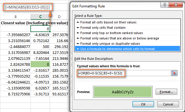
2. b. Creating Custom Rules: To create custom rules, click on the “New Rule” button in the “Conditional Formatting” dialog box. Select the type of rule you want to create and enter your criteria. Choose a formatting style and click “OK.”

Advanced Conditional Formatting Techniques

Excel’s conditional formatting feature also supports more advanced techniques, such as using nested IF statements and combining multiple rules.

a. Using Nested IF Statements in Conditional Formatting: You can use nested IF statements to evaluate multiple conditions in a single rule. For example, you might use an IF statement to check whether a cell’s value is greater than 10, and another IF statement to check whether it is less than 20.

Best Practices for Using Conditional Formatting in Excel

To get the most out of Excel’s conditional formatting feature, it’s important to follow some best practices. Here are a few tips:

• Use conditional formatting sparingly: Too much conditional formatting can make your spreadsheet hard to read and slow to load.
• Keep it simple: Try to use simple formulas and formatting options whenever possible.
• Use color effectively: Choose colors that make sense for the data you’re working with and avoid using too many colors in one spreadsheet.
• Test your rules: Make sure your rules are working as intended by testing them with different data sets.

Conclusion

Conditional formatting is a powerful tool in Microsoft Excel that allows you to format cells based on specific criteria. By using formulas and custom rules, you can highlight important information and make your spreadsheets easier to read. Remember to use best practices when working with conditional formatting, and always test your rules to ensure they’re working correctly.

FAQs

Q: Can I use conditional formatting in Excel to format an entire row based on a cell’s value?

A: Yes, you can use conditional formatting to format an entire row based on a cell’s value. To do this, select the entire row, and use a formula that references the cell you want to evaluate.

Q: How can I create a custom rule that highlights cells that are within a certain date range?

A: To create a custom rule that highlights cells within a date range, use the “A Date Occurring” option in the “Conditional Formatting” dialog box. Choose “Between” and enter your date range.

Q: Can I use conditional formatting to create a data bar that shows the relative value of each cell in a range?

A: Yes, you can use the “Data Bars” option in the “Conditional Formatting” dialog box to create a data bar that shows the relative value of each cell in a range.

Q: Can I use conditional formatting to highlight cells based on their font color?

A: No, conditional formatting in Excel can only evaluate cell values, not font colors.

Q: Can I copy conditional formatting rules from one cell to another?

A: Yes, you can copy conditional formatting rules from one cell to another by using the “Format Painter” tool or by copying and pasting the cell with the formatting rule applied.

Tags: #ExcelCharts #ExcelDashboard #ExcelFormulas #ExcelFunctions #ExcelTemplates #ExcelTipsAndTricks #ExcelTutorials