When working with Excel data, you must know about the AGGREGATE function. This function is used to apply one of 20 different functions across a range of cells and is useful for everything from finding the average of a range of cells to counting the number of cells that contain error values. In this post, we’ll look at how to use the AGGREGATE function and some of the things it can do.

1. The AGGREGATE function is a built-in function in Excel that allows you to apply functions such as SUM, AVERAGE, COUNT, MAX, and MIN to a range of cells or an entire column or row.
2. You can use the AGGREGATE function to calculate measures such as standard deviation, variance, percentage change, etc.
   

Here are some of the functions that AGGREGATE can be used for:

1. Average of values in a range.
2. Maximum of values in a range.
3. Minimum of values in a range.
4. Sum of values in a range.
5. Count the number of cells that contain numbers in a range.
6. Count the number of cells that contain dates in a range.

The AGGREGATE function is used to apply one of 20 different functions across a range of cells.

The AGGREGATE function is a great way to apply one of 20 different functions across a range of cells. This can be extremely helpful when trying to find the average, max, min, or sum of a range of data. The AGGREGATE function is also very user-friendly and easy to use. Simply select the cells you want to aggregate and the type of function you would like to apply from the list of options.

These functions include sum, average, count, maximum, minimum, and more. The syntax is as follows:

=AGGREGATE(value1, {function1}, {argument1}, {function2}, {argument2}, …)

The following table provides a list of functions you can apply using the AGGREGATE command. The first column provides a brief description of each function. The second column contains the syntax for applying each function.

Also, the syntax of the AGGREGATE function is as follows:

=AGGREGATE(function_num, ref, range)

In the above syntax:

The function_num argument must be an integer between 1 and 20. This represents which function will be applied to each cell in the range. ref is the range of cells that is to be applied. the range is the range of cells for which aggregate functions will be performed.

AGGREGATE is useful for finding the average of a range of cells, counting the number of cells that contain error values, and more.

Named for its function, the AGGREGATE Excel function is a great way to find averages of ranges of cells. In addition, it can come in handy for counting the number of cells that contain error values. As you might guess, this can be very useful for debugging your formulas!

To use AGGREGATE, you need to specify the function you want to use (e.g., Average, Count, Max, Min) and the range of cells you want to apply it to.

The AGGREGATE function in Excel is a versatile tool that can perform calculations on various cells. To use AGGREGATE, you need to specify the function you want to use (e. g., Average, Count, Max, Min), as well as the range of cells you want to apply it to. For example, let’s say you have a worksheet with data on students’ test scores.

AGGREGATE can be used with built-in functions or custom functions written

I will show you how to use the AGGREGATE function in Excel. This function is useful if you want to apply a built-in or custom function to a range of cells. You can specify which cells you want the function to ignore and what order your results are in. Let’s take a look at how this works with a simple example.

Example

In this topic, we will focus on the Aggregate/Addition function, which allows us to perform operations such as Addition, Counting, Max, and Min on columns containing error values ​​and hidden cells. This function, which has similar features to subtotals, allows us to operate with cell ranges containing error values, unlike subtotals.

This function has two uses. Reference Format and Array format. Don’t worry about this part; you will already know which format you should use according to your desired transaction inputs. We will clarify this part with the following examples.

Reference format: AGGREGATE (function_num; options; ref1; ref2 ; …)

AGREEMENT(function_num, options, ref1, [ref2],..)

Array format: AGGREGATE (function_num; options; array; k)

AGREEMENT(function_num, options, array, [k])

Here are the key entries:

Function_num: The code of the operation you want to perform.

Options: What should we ignore when making a transaction? (such as error values and hidden cells)

We will need to enter code numbers for both parts, which will be listed in front of us as we write the formula. So let’s look at the use of the function through an example.

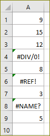
Example 1: What is the sum of the values ​​in the following cell range?

=Aggregate(9,6,A1:A9)

 

To conclude, the SUM function is about conditional formatting bounds. Data bars, Icon Sets, and Color Scales cannot display conditional formatting if the range has errors. This is caused by the MIN, MAX, and PERCENTILE functions failing to calculate when there is an error in the calculation range. The LARGE, SMALL, and STDEVP functions also affect the appropriate functions of some conditional formatting rules for the same reasons. You can apply these functions by using the SUM function as errors will be ignored. In addition, you can apply different aggregation functions to the list or database with the AGREEMENT function, the option to ignore hidden rows and error values.

Tags: Artificial Intelligence Cybersecurity Excel Excel functions leadership PMBOK Guide software development