AVERAGE Function in Excel [2 Easy Way]
What is the AVERAGE Function in Excel? If you are like me and use Excel on a regular basis, then you have probably utilized the AVERAGE function at some point or another. The AVERAGE function is one of the most basic functions in Excel, and it is used to calculate the average value of a given range of cells. In this blog post, we will look at how to use the AVERAGE function in Excel and some practical applications for it. Stay tuned!
Table of Contents
Do you ever need to calculate the average of a series of numbers? Excel’s AVERAGE function makes this easy. You simply input the numbers that you want to average, and Excel does all the work for you. This function can be used in any type of spreadsheet, making it a versatile tool for any situation. Learning how to use the AVERAGE function can help you save time and effort when working with data. Check out this tutorial to learn more!
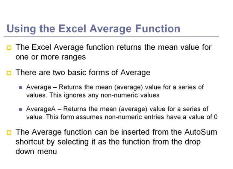
1. What the AVERAGE function is and what it does
2. How to use the AVERAGE function in Excel
3. Some tips and tricks for using the AVERAGE function in Excel
4. Examples of how to use the AVERAGE function in Excel
1. What the AVERAGE function is and what it does
The AVERAGE function is a built-in function in Excel that is used to calculate the average of a given range of cells. The function can be used in any type of spreadsheet, making it a versatile tool for any situation. Excel will automatically calculate the average of the numbers that you input into the function. You can input numbers manually or by selecting a range of cells.
2. How to use the AVERAGE function in Excel
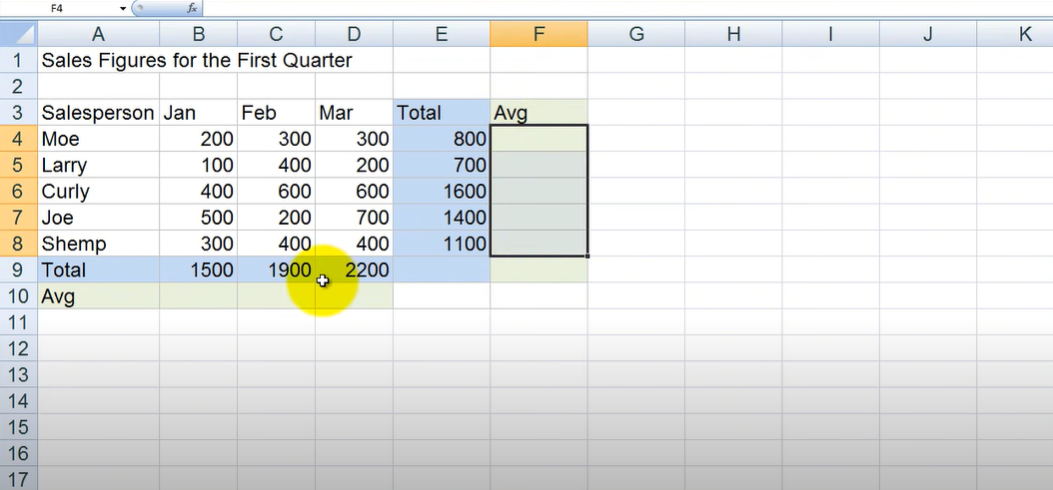
To use the AVERAGE function, follow these steps:
1. Enter the numbers that you want to average into a cell or range of cells.
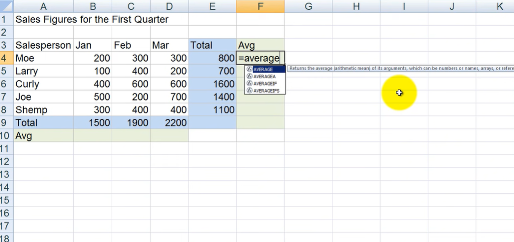
2. Type =AVERAGE( into the cell where you want the result to appear.
3. Select the cells containing the numbers you want to average.
4. Press Enter.
Excel will now calculate the average of the numbers that you selected and display the result in the cell where you entered the function.
If you are like me and use Excel on a regular basis, then you have probably utilized the AVERAGE function at some point or another.
3. Some tips and tricks for using the AVERAGE function in Excel
One tip for using the AVERAGE function is to ensure that all of the cells you want to include in the calculation are adjacent. This will make it easier to select them when you are entering the function. Another tip is to use named ranges when working with large data sets. This can help you track which cells belong in the calculation and make it easier to select them. Let’s take a look at an example of how to use the AVERAGE function. Say we have a list of students’ grades and want to calculate the average grade. We can do this by using the AVERAGE function.
4. Examples of how to use the AVERAGE function in Excel
1. First, we will input the grades into a cell or range of cells.
2. Next, we will type =AVERAGE( into the cell where we want the result to appear.
3. Then, we will select the cells that contain the grades that we want to average.
4. Finally, we will press Enter.
Excel will now calculate the average grade and display the result in the cell where we entered the function. Easy, right?
How to Calculate Averages in Excel 5 Easy Way!
There are a few different ways to calculate averages in Excel. The AVERAGE function is the most straightforward, but there are also some other options that might be better suited for your data. It is the simplest way to calculate an average in Excel. Just enter the range of cells that you want to average, and Excel will do the rest. For example, let’s say we have a list of test scores in column A, and we want to find the average. We would simply enter =AVERAGE(A1:A10) into any cell, and Excel would give us the answer.
If you are like me and use Excel regularly, then you have probably utilized the AVERAGE function at some point or another.
Other Ways to Calculate Averages in Excel
If you have a list of numbers that are not evenly spaced, you might want to use the AVERAGEIF function. This function lets you specify criteria and only the cells that meet that criteria will be averaged. For example, let’s say we have a list of test scores in column A, and we want to find the average for only the scores that are above 80. We would enter =AVERAGEIF(A1:A10,”>80″) into any cell, and Excel would give us the answer.
If you have a lot of data, you might want to use the AVERAGEIFS function. This function is similar to AVERAGEIF, but it lets you specify multiple criteria. For example, let’s say we have a list of test scores in column A, and we want to find the average for only the scores that are above 80 and below 90. We would enter =AVERAGEIFS(A1:A10,”>80″,”<90″) into any cell, and Excel would give us the answer. No matter which method you use, calculating averages in Excel is easy! Just remember to use the AVERAGE function for simple data sets, the AVERAGEIF function for data sets that are not evenly spaced, and the AVERAGEIFS function for data sets with multiple criteria.
There are many applications for the AVERAGE function in Excel. You can use it to calculate things like class grades, test scores, sales totals, and more. The AVERAGE function is a quick and easy way to get the information that you need.
I hope this blog post has been helpful in understanding how to use the AVERAGE function in Excel. If you have any questions, please leave a comment below. Thanks for reading!
Hello, I’m Cansu, a professional dedicated to creating Excel tutorials, specifically catering to the needs of B2B professionals. With a passion for data analysis and a deep understanding of Microsoft Excel, I have built a reputation for providing comprehensive and user-friendly tutorials that empower businesses to harness the full potential of this powerful software.
I have always been fascinated by the intricate world of numbers and the ability of Excel to transform raw data into meaningful insights. Throughout my career, I have honed my data manipulation, visualization, and automation skills, enabling me to streamline complex processes and drive efficiency in various industries.
As a B2B specialist, I recognize the unique challenges that professionals face when managing and analyzing large volumes of data. With this understanding, I create tutorials tailored to businesses’ specific needs, offering practical solutions to enhance productivity, improve decision-making, and optimize workflows.
My tutorials cover various topics, including advanced formulas and functions, data modeling, pivot tables, macros, and data visualization techniques. I strive to explain complex concepts in a clear and accessible manner, ensuring that even those with limited Excel experience can grasp the concepts and apply them effectively in their work.
In addition to my tutorial work, I actively engage with the Excel community through workshops, webinars, and online forums. I believe in the power of knowledge sharing and collaborative learning, and I am committed to helping professionals unlock their full potential by mastering Excel.
With a strong track record of success and a growing community of satisfied learners, I continue to expand my repertoire of Excel tutorials, keeping up with the latest advancements and features in the software. I aim to empower businesses with the skills and tools they need to thrive in today’s data-driven world.
Suppose you are a B2B professional looking to enhance your Excel skills or a business seeking to improve data management practices. In that case, I invite you to join me on this journey of exploration and mastery. Let’s unlock the true potential of Excel together!
https://www.linkedin.com/in/cansuaydinim/

